Understanding SCTE-35

Introduction

SCTE-35 is a standard to signal an advertisement (ad) insertion opportunity in a transport stream. This relatively short standard document is, however, difficult to understand without the insight of ad insertion workflow. This article explains the standard text with some background and context information.

Most TV programs make money by selling ad time slots to the advertisers. For example, 30 second ad time slot of Super Bowl 2014 was sold for $4 million.

Ads are not hard coded into the TV program. Instead, the broadcasters insert the ad to the time slot on the fly. This allows broadcasters to change ad based on the air time, geographic location, or even personal preference. All we need is a special marker in the broadcast stream to signal the ad time slots.

Network program and advertisement.

Analog broadcasting used a special audio tone called DTMF to signal the ad time slot. In digital broadcasting, we use SCTE-35.

SCTE-35 packets are multiplexed with video and audio packets in the transport stream. The syntax of the payload is called splice_info_section(). The syntax signals one of six commands. The most important command is splice_insert() and I explain it first.

Splice Insert Command

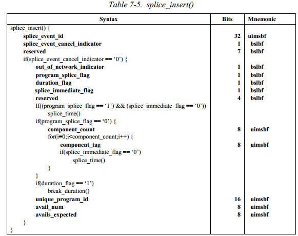
splice_insert_syntax

splice_insert signals a splice event. When out_of_network_indicator is 1, it signals switching from the network program to an advertisement. When out_of_network_indicator is 0, it signals switching back to the network program. Although not formally defined in the standard, these events are often called cue-out event and cue-in event respectively.

splice_event

The timing of the splice event is specified in terms of PTS. It uses two fields; pts_adjustment field in splice_info_section() syntax and pts_time field in splice_insert() syntax. The splice event PTS is calculated as (pts\_time + pts\_adjustment) \mod{M} where M is PTS rollover modulo: 2^{33}. In practice, pts_time field often carries relative PTS from the network program start. When broadcasting the program, the edge multiplexer sets the current PTS offset in pts_adjustment so that the resultant event PTS is aligned with the broadcast time base.

Many ad time slots have a fixed duration such as 15, 30, and 45 seconds. Instead of explicitly signaling cue-in event, you can use break_duration() syntax to specify duration of the time slot in the cue-out event. When auto_return field is 0, the signaled duration is interpreted as “informative” and you still have to signal cue-in event. When auto_return field is 1, the devices terminates the break after the specified duration without a cue-in event. Note that you can always overwrite the break duration by signaling cue-in event explicitly.

It is also possible to signal a splice event without specifying the time. When splice_immediate_flag is 1, a splice event is triggered at the earliest possible timing. This, however, causes various headaches in practice. For example, when you have redundant systems to produce same broadcast streams, “Immediate” might result in slightly different timing on each system due to the command delivery latency. SCTE-35 recommends to use splice_immediate_flag = 1 only for early termination of ad breaks.

Splice Schedule Command

Another command to explain is splice_schedule(). It has similar syntax and semantic as splice_insert() but it uses wallclock time instead of PTS. This allows to schedule the ad breaks far before the actual event based on the broadcast schedule and wall clock time. On the other hand, wallclock time has only second precision and not suitable for frame accurate splicing.

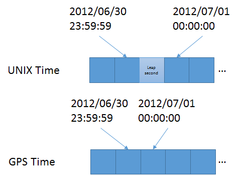
It is worth noting that the wallclock time uses so called GPS time. For engineers who are familiar with C/C++ time function such as time(), GPS time is different in two important ways.

  1. The epoch is 1980/01/06T00:00:00Z instead of 1970/01/01T00:00:00Z.
  2. Leap seconds are counted instead of skipped. As of today, there are 16 leap seconds since 1980/01/06. Therefore, GPS time looks 16 seconds ahead of the wall clock time we are familiar with.

leap_second

The leap second problem can be hard in some use cases. Since leap second is unpredictable, we need to look up the latest leap second information published by IERS. A correct way is to read GPS_UTC_offset value encoded in PSIP metadata carried in ATSC stream. However, not every system has access to the information. SCTE-35 allows implementation to ignore the leap second but it results in about 16 second error.

Splice Event Repetition and Cancellation

Both splice_insert and splice_schedule commands are issued with a unique identifier of each splice event. The identifier is 32 bit integer and usually incremented for each event.

splice_event_id

You might wonder how to ensure the uniqueness of splice_event_id for long running 24/7 live event. It is 32 bits integer. Even if we have splice event for every second, we won’t running out of the number for 2^{32} / 60 / 60 / 24 / 365 = 136 years. We are good.

One use case of splice_event_id is redundant repetition. As transport stream packets are often delivered over unreliable network, it is recommended to send splice_insert command multiple times with a same splice_event_id before the actual event. Another use case is a cancellation. You can cancel an event by specifying the splice_event_id and set splice_event_cancel_indicator to 1. You can also override an event by inserting a new one after cancellation. To prevent a race condition, it is required to finalize the splice_event 4 second before the actual event.

Segmentation

SCTE-35 was originally designed for ad insertion. However, it turned out to be also useful for more general segmentation signaling.

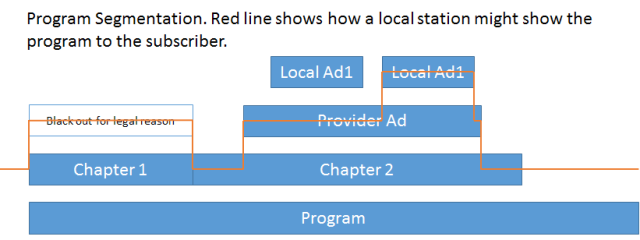
Consider a movie program. The program may have one or more “chapters” as you see on DVD. Some parts of the program are reserved for provider ads such as announcement of TV drama to broadcast tonight. Within that time slot, some parts may be reserved for the local ads.

Depending on the distribution method (TV, Web, DVR recording, etc), the provider may want to make only the selected part of the program available for legal reasons.

Also, each segment may have associated identifier such as TMS ID, AD-ID, and ATSC content identifier. These identifiers are collectively called UPID (Unique Program Identifier) and would be useful for content management purpose.

program_segmentation

Such hierarchical structure cannot be signaled by splice_insert syntax. Also, splice_insert is not sufficient to carry various metadata such as restrictions and UPID. The SCTE-35 segmentation descriptor addresses the problem.

Segmentation is signaled by a combination of time_signal command and segmentaiton_descriptor. The time_signal command simply signals a timestamp of the segmentation.

time_signal

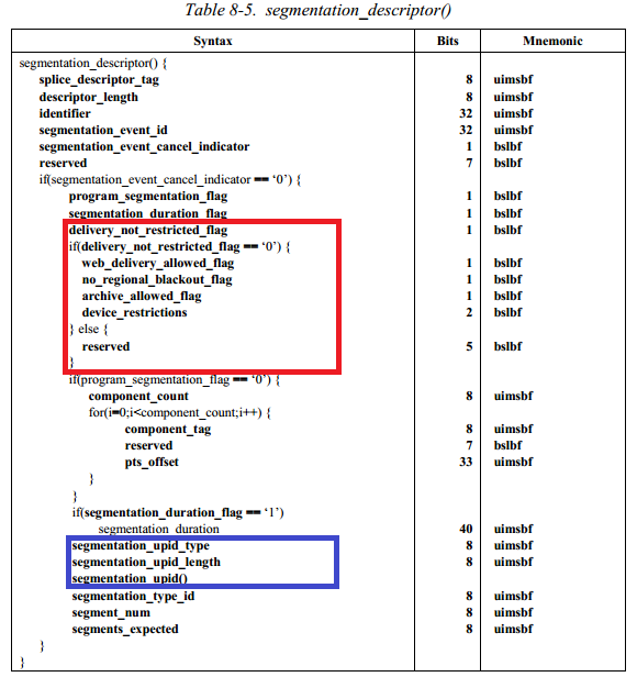
The complex matter is all taken care by segment descriptor.

segmentation_descriptor

The red part describes various restrictions based on the delivery method. For example, you can make the segment not available for Web delivery.

The blue part carries UPID which identifies the content of the segment. For example, you can identify a segment to be “Gone with the wind” by looking up UPID (ISAN number) encoded in the SCTE-35 message.

The structure of segmentation is similar to splice event except one important difference. In splice event, splice_event_id identifies each splice event, i.e. cue-out and cue-in have different splice_event_id. On the other hand, segmentation_event_identifier identifies one entire segment. This allows segments to be nested and make hierarchical structure.

segmentation_event_id

SCTE-35 on over the top delivery

SCTE-35 is specific to a transport stream which is mainly used for traditional broadcasting context. As Web based video delivery becomes popular, many companies try to make something similar to SCTE-35 for Web delivery. For example, one attempt can be seen in a proprietary extension to HLS media playlist m3u8 format for ad insertion.

Although it is difficult to predict the future, I think all these proprietary ad marker technologies are to be faded out and the industry trends is moving in favor of using SCTE-35 as the ad marker data model. For example, a company uses XML representation of SCTE-35 as Web video ad marker. Another company uses base-64 encoded SCTE-35 splice_info_section syntax as an adaptive bit rate streaming ad marker. This is because they don’t want to lose any information of SCTE-35, which is matured and well supported by various devices, on the way from the content management system to cable network to Web delivery.

Posted in Video | Tagged , , | 27 Comments

Regression bug!? Hold a moment…

It was a quiet Friday until a QA guy shouted “Hey, we just hit a showstopper problem!”

The problem was difficult to reproduce, which, say, only 5% of trials resulted in the failure. In the follow up test, QA installed a previous version of the software and ran 30 times but they couldn’t reproduce. Now, can we conclude it is a regression bug?

Not really. Even if the previous version has the bug, it may not fail just by luck. Let’s do the math.

The probability of zero failure in 30 trials when the underlying failure rate is 5% follows binomial distribution, which is \binom{30}{0}\times 0.05^{0} \times (1-0.05)^{30} = 0.215. It means we still have more than 20% chance of the bug existing also in the previous version.

To reasonably conclude a regression bug, we may want to reduce the chance to less than 5%. To get that level, we need 59 trials because

\binom{58}{0}\times 0.05^{0} \times (1-0.05)^{58} = 0.051

\binom{59}{0}\times 0.05^{0} \times (1-0.05)^{59} = 0.048

Posted in Statistics | Leave a comment

Condition variables performance of boost, Win32, and the C++11 standard library

About four years ago, I wrote the condition variables in Win32 API was much faster than boost threading library implementation. Since then the boost threading library has been rewritten and C++11 has introduced the threading support in the standard library. Let’s revisit the benchmark again.
The test program is bounded FIFO implemented with two condition variables. It passes 10,000,000 integers from the producer to the consumer. The test is conducted 50 times with the following environment.

– Intel(R) Core (TM) i7 950@3GHz.
– Windows 7 Professional
– Visual Studio 2012 Express (Update 1)

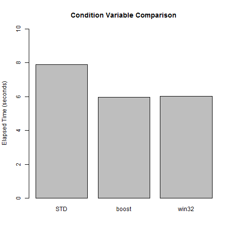
The average speed is shown here. Shorter is faster. Notice that it’s the result of 10 million times FIFO access. Although std::condition_variable is slower than others, the difference is pretty much nothing.

cv_comp_average

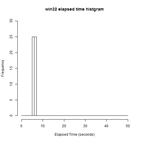
However, the distributions of elapsed time are still interesting. Among 50 times trial, Win32 and boost condition variables have pretty stable performance.

cv_comp_boost_dist

cv_comp_win32_dist

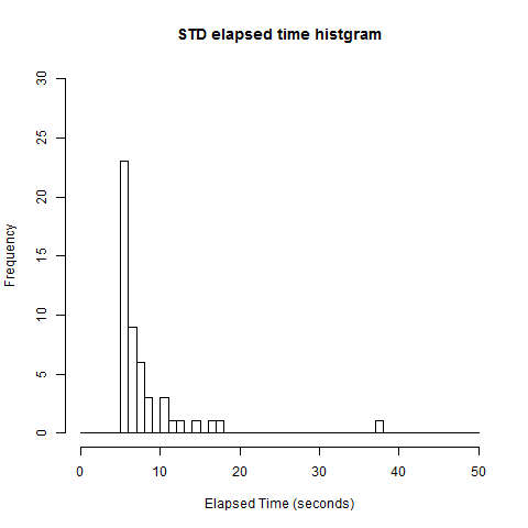
For unknown reason, however, std::condition_variable of Visual Studio 2012 Update 1 implementation sometimes takes very long time.

cv_comp_std_dist

Here is the test program.

#include <boost/thread.hpp>
#include <boost/timer.hpp>
#include <deque>
#include <thread>
#include <mutex>
#include <condition_variable>
#include <windows.h>

using namespace std;

class fifo
{
public:
    virtual ~fifo(){}
    virtual void push(int v) = 0;
    virtual int  pull()      = 0;
};

class boost_fifo : public fifo
{
public:
    boost_fifo(std::size_t s) : max_fifo_size(s){}

    void push(int v)
    {
        boost::mutex::scoped_lock lk(mtx);
        while(buffer.size() > max_fifo_size)
        {
            cv_slot.wait(lk);
        }
        buffer.push_back(v);
        cv_data.notify_one();
    }

    int pull()
    {
        boost::mutex::scoped_lock lk(mtx);
        while(buffer.empty())
        {
            cv_data.wait(lk);
        }
        int v = buffer.front();
        buffer.pop_front();
        cv_slot.notify_one();
        return v;
    }
private:
    std::size_t max_fifo_size;
    boost::mutex mtx;
    boost::condition_variable cv_slot;
    boost::condition_variable cv_data;
    std::deque<int> buffer;
};

class win32_fifo : public fifo
{
public:
    win32_fifo(std::size_t s) : max_fifo_size(s)
    {
        InitializeCriticalSection(&mtx);
        InitializeConditionVariable(&cv_slot);
        InitializeConditionVariable(&cv_data);
    }

    ~win32_fifo()
    {
        DeleteCriticalSection(&mtx);
    }

    void push(int v)
    {
        EnterCriticalSection(&mtx);
        while(buffer.size() > max_fifo_size)
        {
            SleepConditionVariableCS(&cv_slot, &mtx, INFINITE);
        }
        buffer.push_back(v);
        WakeConditionVariable(&cv_data);
        LeaveCriticalSection(&mtx);
    }

    int pull()
    {
        EnterCriticalSection(&mtx);
        while(buffer.empty())
        {
            SleepConditionVariableCS(&cv_data, &mtx, INFINITE);
        }

        int v = buffer.front();
        buffer.pop_front();
        WakeConditionVariable(&cv_slot);
        LeaveCriticalSection(&mtx);
        return v;
    }
private:
    std::size_t max_fifo_size;
    CRITICAL_SECTION mtx;
    CONDITION_VARIABLE cv_slot;
    CONDITION_VARIABLE cv_data;
    std::deque<int> buffer;
};

class std_fifo : public fifo
{
public:
    std_fifo(std::size_t s) : max_fifo_size(s){}

    void push(int v)
    {
        std::unique_lock<std::mutex> lk(mtx);
        while(buffer.size() > max_fifo_size)
        {
            cv_slot.wait(lk);
        }
        buffer.push_back(v);
        cv_data.notify_one();
    }

    int pull()
    {
        std::unique_lock<std::mutex> lk(mtx);
        while(buffer.empty())
        {
            cv_data.wait(lk);
        }
        int v = buffer.front();
        buffer.pop_front();
        cv_slot.notify_one();
        return v;
    }
private:
    std::size_t max_fifo_size;
    std::mutex mtx;
    std::condition_variable cv_slot;
    std::condition_variable cv_data;
    std::deque<int> buffer;
};

void push_loop(fifo* fifo_buffer)
{
    for(int i = 0; i < 10000000; i++)
    {
        fifo_buffer->push(i);
    }
}

void pull_loop(fifo* fifo_buffer)
{
    for(int i = 0; i < 10000000; i++)
    {
        fifo_buffer->pull();
    }
}

int main()
{
    vector<double> elapsedTime[3];
    
    static size_t const FIFO_SIZE = 16;
    for(int i = 0; i < 50; i++)
    {
        cerr << "BOOST FIFO: " << endl;
        {
            boost::timer tim;
            unique_ptr<fifo> fifo_buffer(new boost_fifo(FIFO_SIZE));
            boost::thread push_thread(bind(push_loop, fifo_buffer.get()));
            boost::thread pull_thread(bind(pull_loop, fifo_buffer.get()));
            
            push_thread.join();
            pull_thread.join();

            elapsedTime[0].push_back(tim.elapsed());
        }

        cerr << "WIN32 FIFO: " << endl;
        {
            boost::timer tim;
            unique_ptr<fifo> fifo_buffer(new win32_fifo(FIFO_SIZE));
            boost::thread push_thread(bind(push_loop, fifo_buffer.get()));
            boost::thread pull_thread(bind(pull_loop, fifo_buffer.get()));
            
            push_thread.join();
            pull_thread.join();
            
            elapsedTime[1].push_back(tim.elapsed());
        }

        cerr << "STD FIFO: " << endl;
        {
            boost::timer tim;
            unique_ptr<fifo> fifo_buffer(new std_fifo(FIFO_SIZE));
            boost::thread push_thread(bind(push_loop, fifo_buffer.get()));
            boost::thread pull_thread(bind(pull_loop, fifo_buffer.get()));
            
            push_thread.join();
            pull_thread.join();
            
            elapsedTime[2].push_back(tim.elapsed());
        }
    }
    
    for(auto v : elapsedTime)
    {
        for(auto e : v)
        {
            cout << e << ", ";
        }
        cout << endl;
    }

    return 1;
}

I used the following R code generate the graph. It also contains the raw data of elapsed time.

std <- c(5.183,  5.701,  7.006,  5.839,  5.524, 16.463,  8.336,  7.041,
         5.574,  5.098,  5.430,  5.034,  5.244,  6.088,  7.478,  5.557,
         5.062,  5.577,  5.266,  5.991,  5.900,  6.804,  6.452,  6.981,
         10.586, 7.152, 37.248,  5.469, 12.113,  6.645,  8.030, 10.559,
         10.695, 6.878,  6.321, 11.659,  6.210, 17.335,  5.804,  6.146,
         5.067,  5.709,  5.938,  5.718,  8.967,  7.143,  5.078,  7.472,
         5.347, 15.000)

boost <- c(6.104, 6.11, 5.862, 5.07, 5.311, 5.639, 5.402, 5.532, 5.61,
           5.686, 6.129, 5.481, 5.07, 5.602, 5.276, 6.046, 5.818, 6.209,
           6.111, 6.165, 5.828, 6.266, 5.806, 6.087, 5.708, 6.119, 6.406,
           6.096, 6.005, 6.332, 6.522, 6.91, 6.921, 5.765, 6.223, 5.444,
           6.274, 6.603, 5.717, 6.471, 5.968, 6.188, 6.608, 5.333, 5.506,
           5.507, 6.241, 5.981, 5.915, 6.515)

win32 <- c(4.356, 5.354, 4.641, 7.821, 4.664, 4.593, 7.174, 5.596, 4.493,
           4.353, 8.678, 4.459, 5.135, 4.526, 5.043, 4.997, 5.148, 5.03,
           7.421, 6.344, 7.64, 5.491, 6.101, 6.054, 6.626, 6.292, 6.29,
           6.912, 5.691, 5.991, 6.263, 6.096, 6.544, 8.024, 6.405, 6.216,
           6.157, 5.821, 7.759, 5.454, 6.364, 8.168, 8.471, 5.108, 6.192,
           5.385, 5.427, 5.855, 6.099, 5.539)

avg <- c(mean(std), mean(boost), mean(win32))

png("cv_comp_average.png")
barplot(avg, main="Condition Variable Comparison", names.arg = c("STD", "boost", "win32"), ylab="Elapsed Time (seconds)", ylim=c(0, 10))
dev.off()

png("cv_comp_std_dist.png")
hist(std, main="STD elapsed time histgram", xlab="Elapsed Time (seconds)", breaks=seq(0, 50, 1.0), ylim=c(0, 30))
dev.off()

png("cv_comp_boost_dist.png")
hist(boost, main="boost elapsed time histgram", xlab="Elapsed Time (seconds)", breaks=seq(0, 50, 1.0), ylim=c(0, 30))
dev.off()

png("cv_comp_win32_dist.png")
hist(boost, main="win32 elapsed time histgram", xlab="Elapsed Time (seconds)", breaks=seq(0, 50, 1.0), ylim=c(0, 30))
dev.off()
Posted in C++, Optimization | Tagged , , | 1 Comment

Make your first HEVC stream

This article shows how to encode your video with HM (HEVC Test Model (HM)), the reference implementation developed by the standard organizations.

HM is provided as a source code so that we can build on various platforms. But let’s focus on Windows and Microsoft Visual Studio tool chain for now.

Step 0: Prerequisite

  1. Microsofot Visual Studio 2008 or later. Express version should work. [Download]
  2. Your favorite YUV viewer such as YUV Player [Download]
  3. Subversion client such as Sliksvn [Download]
  4. Sample YUV file such as this [Download]

Step 1: Download the source tree

Get the latest version of HM.

% svn co https://hevc.hhi.fraunhofer.de/svn/svn_HEVCSoftware/trunk

Step 2: Build it!

Start Visual Studio command line prompt and build HM_vc9.sln located in trunk/build directory.
% msbuild /p:Configuration=Release HM_vc9.sln

Step 3: Encode it!

Open a notepad and make a configuration text file as shown at the bottom of this article. Save it as test.config. The encoder tool is called TAppEncoder.exe which should be located in trunk/bin/vc9/win32/release.
% TAppEncoder.exe -c test.cfg -i mobile_cif.yuv

Step 4: Check the output

The step above encodes the first 10 frames at 100kbps and creates mobile.hevc, which is your first HEVC stream. Congratulations!

The encoding tool also conveniently made YUV file which was decoded from the HEVC stream. You can compare the original (mobile_cif.yuv) and encoded file (mobile_out.yuv).

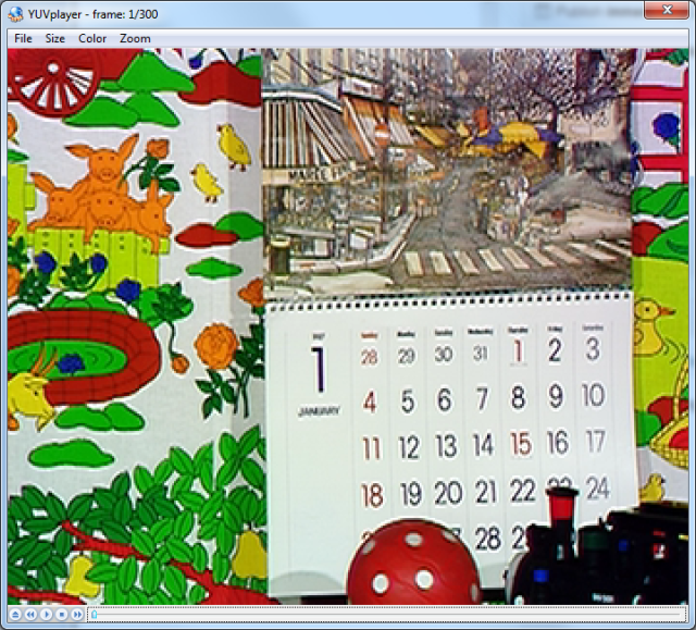
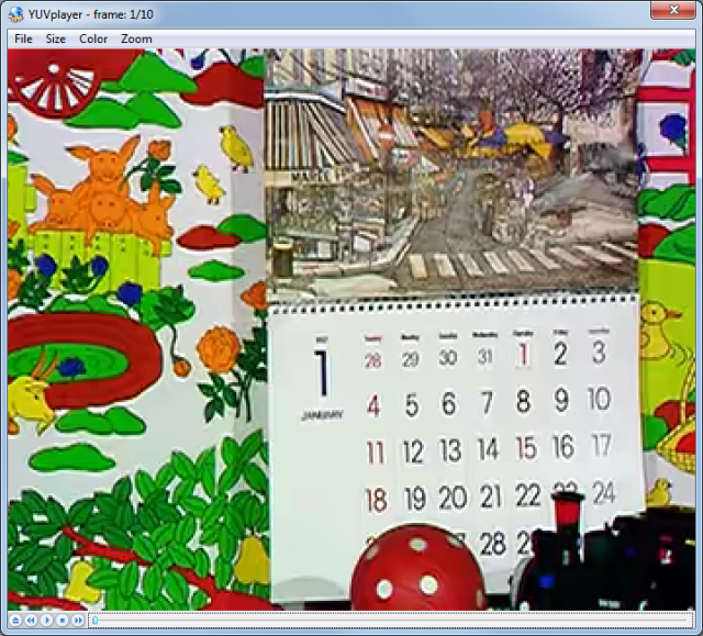
This is the original frame.

This is the encoded frame.

Do you see the difference? It’s doing pretty good job for 100kbps – but you can see some compression artifact here.

Configuration file

Here is the configuration file I used. Hover the mouse to right-top area to copy it.

Update: The config file was updated to the latest HM (Feb 6, 2013)

#======== File I/O =====================
BitstreamFile                 : mobile.hevc
ReconFile                     : mobile_out.yuv

FrameRate                     : 24          # Frame Rate per second
FrameSkip                     : 0           # Number of frames to be skipped in input
SourceWidth                   : 352         # Input  frame width
SourceHeight                  : 288         # Input  frame height
FramesToBeEncoded             : 10          # Number of frames to be coded

#======== Unit definition ================
MaxCUWidth                    : 64          # Maximum coding unit width in pixel
MaxCUHeight                   : 64          # Maximum coding unit height in pixel
MaxPartitionDepth             : 4           # Maximum coding unit depth
QuadtreeTULog2MaxSize         : 5           # Log2 of maximum transform size for
                                            # quadtree-based TU coding (2...6)
QuadtreeTULog2MinSize         : 2           # Log2 of minimum transform size for
                                            # quadtree-based TU coding (2...6)
QuadtreeTUMaxDepthInter       : 3
QuadtreeTUMaxDepthIntra       : 3

#======== Coding Structure =============
IntraPeriod                   : -1          # Period of I-Frame ( -1 = only first)
DecodingRefreshType           : 0           # Random Accesss 0:none, 1:CDR, 2:IDR
GOPSize                       : 4           # GOP Size (number of B slice = GOPSize-1)
#        Type POC QPoffset QPfactor tcOffsetDiv2 betaOffsetDiv2  temporal_id #ref_pics_active #ref_pics reference pictures predict deltaRPS #ref_idcs reference idcs 
Frame1:  B    1   3        0.4624   0            0               0           4                4         -1 -5 -9 -13       0
Frame2:  B    2   2        0.4624   0            0               0           4                4         -1 -2 -6 -10       1      -1       5         1 1 1 0 1
Frame3:  B    3   3        0.4624   0            0               0           4                4         -1 -3 -7 -11       1      -1       5         0 1 1 1 1            
Frame4:  B    4   1        0.578    0            0               0           4                4         -1 -4 -8 -12       1      -1       5         0 1 1 1 1
ListCombination               : 1           # Use combined list for uni-prediction in B-slices

#=========== Motion Search =============
FastSearch                    : 1           # 0:Full search  1:TZ search
SearchRange                   : 64          # (0: Search range is a Full frame)
BipredSearchRange             : 4           # Search range for bi-prediction refinement
HadamardME                    : 1           # Use of hadamard measure for fractional ME
FEN                           : 1           # Fast encoder decision
FDM                           : 1           # Fast Decision for Merge RD cost

#======== Quantization =============
QP                            : 32          # Quantization parameter(0-51)
MaxDeltaQP                    : 0           # CU-based multi-QP optimization
MaxCuDQPDepth                 : 0           # Max depth of a minimum CuDQP for sub-LCU-level delta QP
DeltaQpRD                     : 0           # Slice-based multi-QP optimization
RDOQ                          : 1           # RDOQ
RDOQTS                        : 1           # RDOQ for transform skip

#=========== Deblock Filter ============
DeblockingFilterControlPresent: 0           # Dbl control params present (0=not present, 1=present)
LoopFilterOffsetInPPS         : 0           # Dbl params: 0=varying params in SliceHeader, param = base_param + GOP_offset_param; 1=constant params in PPS, param = base_param)
LoopFilterDisable             : 0           # Disable deblocking filter (0=Filter, 1=No Filter)
LoopFilterBetaOffset_div2     : 0           # base_param: -13 ~ 13
LoopFilterTcOffset_div2       : 0           # base_param: -13 ~ 13

#=========== Misc. ============
InternalBitDepth              : 8           # codec operating bit-depth

#=========== Coding Tools =================
SAO                           : 1           # Sample adaptive offset  (0: OFF, 1: ON)
AMP                           : 1           # Asymmetric motion partitions (0: OFF, 1: ON)
TransformSkip                 : 1           # Transform skipping (0: OFF, 1: ON)
TransformSkipFast             : 1           # Fast Transform skipping (0: OFF, 1: ON)
SAOLcuBoundary                : 0           # SAOLcuBoundary using non-deblocked pixels (0: OFF, 1: ON)

#============ Slices ================
SliceMode                : 0                # 0: Disable all slice options.
                                            # 1: Enforce maximum number of LCU in an slice,
                                            # 2: Enforce maximum number of bytes in an 'slice'
                                            # 3: Enforce maximum number of tiles in a slice
SliceArgument            : 1500             # Argument for 'SliceMode'.
                                            # If SliceMode==1 it represents max. SliceGranularity-sized blocks per slice.
                                            # If SliceMode==2 it represents max. bytes per slice.
                                            # If SliceMode==3 it represents max. tiles per slice.

LFCrossSliceBoundaryFlag : 1                # In-loop filtering, including ALF and DB, is across or not across slice boundary.
                                            # 0:not across, 1: across

#============ PCM ================
PCMEnabledFlag                      : 0                # 0: No PCM mode
PCMLog2MaxSize                      : 5                # Log2 of maximum PCM block size.
PCMLog2MinSize                      : 3                # Log2 of minimum PCM block size.
PCMInputBitDepthFlag                : 1                # 0: PCM bit-depth is internal bit-depth. 1: PCM bit-depth is input bit-depth.
PCMFilterDisableFlag                : 0                # 0: Enable loop filtering on I_PCM samples. 1: Disable loop filtering on I_PCM samples.

#============ Tiles ================
UniformSpacingIdc                   : 0                # 0: the column boundaries are indicated by ColumnWidth array, the row boundaries are indicated by RowHeight array
                                                       # 1: the column and row boundaries are distributed uniformly
NumTileColumnsMinus1                : 0                # Number of columns in a picture minus 1
ColumnWidthArray                    : 2 3              # Array containing ColumnWidth values in units of LCU (from left to right in picture)   
NumTileRowsMinus1                   : 0                # Number of rows in a picture minus 1
RowHeightArray                      : 2                # Array containing RowHeight values in units of LCU (from top to bottom in picture)

LFCrossTileBoundaryFlag           : 1                  # In-loop filtering is across or not across tile boundary.
                                                       # 0:not across, 1: across 

#============ WaveFront ================
WaveFrontSynchro                    : 0                # 0:  No WaveFront synchronisation (WaveFrontSubstreams must be 1 in this case).
                                                       # >0: WaveFront synchronises with the LCU above and to the right by this many LCUs.

#=========== Quantization Matrix =================
ScalingList                   : 0                      # ScalingList 0 : off, 1 : default, 2 : file read
ScalingListFile               : scaling_list.txt       # Scaling List file name. If file is not exist, use Default Matrix.

#============ Lossless ================
TransquantBypassEnableFlag: 0  # Value of PPS flag.
CUTransquantBypassFlagValue: 0 # Constant lossless-value signaling per CU, if TransquantBypassEnableFlag is 1.

#============ Rate Control ======================
RateControl                         : 0                # Rate control: enable rate control
TargetBitrate                       : 1000000          # Rate control: target bitrate, in bps
KeepHierarchicalBit                 : 1                # Rate control: keep hierarchical bit allocation in rate control algorithm
LCULevelRateControl                 : 1                # Rate control: 1: LCU level RC; 0: picture level RC
RCLCUSeparateModel                  : 1                # Rate control: use LCU level separate R-lambda model
InitialQP                           : 0                # Rate control: initial QP
RCForceIntraQP                      : 0                # Rate control: force intra QP to be equal to initial QP

### DO NOT ADD ANYTHING BELOW THIS LINE ###
### DO NOT DELETE THE EMPTY LINE BELOW ###
Posted in Video | Tagged , , | 134 Comments

Find the MPEG output order from decoding order

Suppose there is a MPEG picture sequence and you know the decoding order. How do you get the output order (=presentation order)?

Assuming every picture is a frame structure, we can use the following method.

Imagine a ditch. Only I or P picture drops into it. If a picture drops when the ditch already has another picture, it’s pushed out. For example, suppose we have a picture sequence in decoding order: I, B, P, I.

The I picture is coming from the left and …

dropped into the ditch.

B picture passes over the ditch and outputs (presented).

P picture drops into the ditch…

And it pushes out the I picture. The I picture outputs.

Then, the last I picture comes. It drops into the ditch …

and pushes out the P picture.

Therefore, the output order is B, I, P. The last I picture stays in the ditch until another reference picture or a sequence_end_code.

The method also indicates several interesting observations.

  1. PTS of a reference picture (I/P) is greater than DTS. DTS is a timestamp when the picture comes from the left. PTS is a timestamp when the picture is pushed out from the ditch.
  2. PTS of a non-Reference picture (B) is same as DTS.
  3. The last output picture is always a reference picture.

When a frame is coded as two field pictures, group each pair to one symbol as shown below.

  • II -> I
  • IP -> I
  • PP -> P
  • BB -> B

Then apply the method. Once you get the output order, convert the symbol back to the original picture types.

This method does not apply for H.264. To get output order of H.264 picture sequence, we need to parse POC (Picture Order Count) information coded in the bit stream.

Posted in Video | Tagged , , , , , | 2 Comments

HEVC – What are CTU, CU, CTB, CB, PB, and TB?

HEVC, also known as H.265 or MPEG-H part 2(ISO/IEC 23008-2), is just around the corner. A good overview was published. The reference implementation is available. Active discussion can be read in the JCT-VC document management system. The Final Draft International Standard (FDIS) is expected be produced in January 2013.

However, as always, the standard writers love cryptic acronyms. Probably the first acronyms which discourage standard readers are block structure coding terminologies, namely CTU, CU, CTB, CB, PB, and TB.

They are basically replacement of Macroblocks and blocks in prior standards. Unlike 10 years ago, we have much higher frame sizes to deal with. 4K production became practical and people start talking about 8K. Even mobile device has higher than HD frame size such as 2048 x 1530. We need larger macroblocks to efficiently encode the motion vectors for these frame size. On the other hand, small detail is still important and we sometimes want to perform prediction and transformation at the granularity of 4×4.

How could we support wide variety of block sizes in efficient manner? That’s a challenge HEVC is trying to solve with those acronyms.

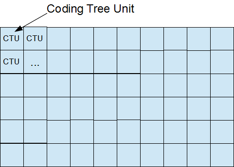
Let’s start from the higher level. Suppose we have a picture to encode. HEVC divides the picture into CTUs (Coding Tree Unit).

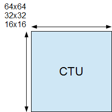
The width and height of CTU are signaled in a sequence parameter set, meaning that all the CTUs in a video sequence have the same size: 64×64, 32×32, or 16×16.

We need to understand an important naming convention here. In HEVC standard, if something is called xxxUnit, it indicates a coding logical unit which is in turn encoded into an HEVC bit stream. On the other hand, if something is called xxxBlock, it indicates a portion of video frame buffer where a process is target to.

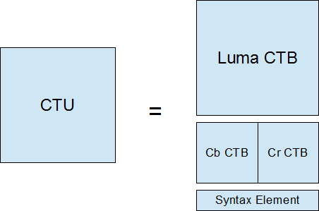
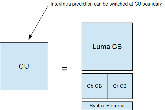
CTU – Coding Tree Unit is therefore a logical unit. It usually consists of three blocks, namely luma (Y) and two chroma samples (Cb and Cr), and associated syntax elements. Each block is called CTB (Coding Tree Block).

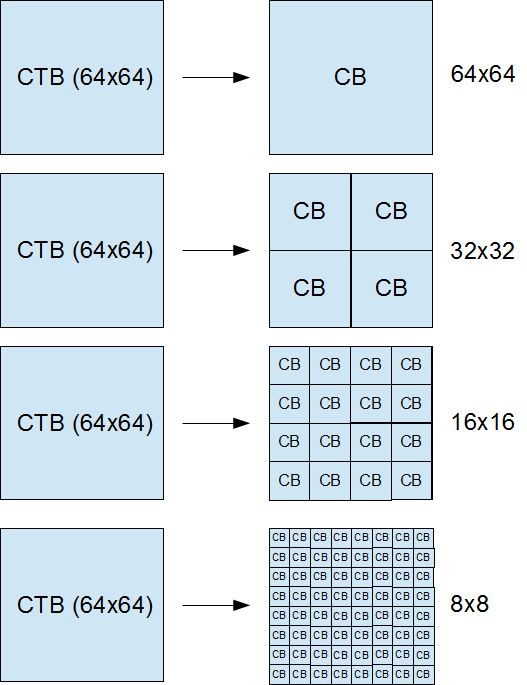
Each CTB still has the same size as CTU – 64×64, 32×32, or 16×16. Depending on a part of video frame, however, CTB may be too big to decide whether we should perform inter-picture prediction or intra-picture prediction. Thus, each CTB can be differently split into multiple CBs (Coding Blocks) and each CB becomes the decision making point of prediction type. For example, some CTBs are split to 16×16 CBs while others are split to 8×8 CBs. HEVC supports CB size all the way from the same size as CTB to as small as 8×8.

The following picture illustrates how 64×64 CTB can be split into CBs.

CB is the decision point whether to perform inter-picture or intra-picture prediction. More precisely, the prediction type is coded in CU (Coding Unit). CU consists of three CBs (Y, Cb, and Cr) and associated syntax elements.

CB is good enough for prediction type decision, but it could still be too large to store motion vectors (inter prediction) or intra prediction mode. For example, a very small object like snowfall may be moving in the middle of 8×8 CB – we want to use different MVs depending on the portion in CB.

Snowfall

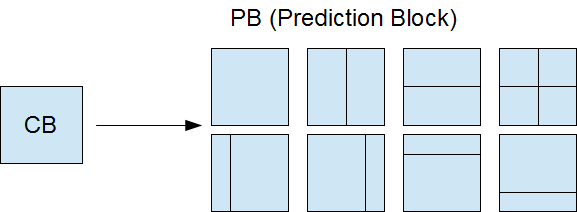
Thus, PB was introduced. Each CB can be split to PBs differently depending on the temporal and/or spatial predictability.

Once the prediction is made, we need to code residual (difference between predicted image and actual image) with DCT-like transformation. Again, CB could be too big for this because a CB may contains both a detailed part (high frequency) and a flat part (low frequency). Therefore, each CB can be differently split into TBs (Transform Block). Note that TB doesn’t have to be aligned with PB. It is possible and often makes sense to perform single transform across residuals from multiple PBs, vise versa.

Let’s read a draft standard text regarding to these terminologies. They should make more sense now.

CTU (coding tree unit): A coding tree block of luma samples, two corresponding coding tree blocks of chroma samples of a picture that has three sample arrays, or a coding tree block of samples of a monochrome picture or a picture that is coded using three separate colour planes and syntax structures used to code the samples. The division of a slice into coding tree units is a partitioning.

CTB (coding tree block): An NxN block of samples for some value of N. The division of one of the arrays that compose a picture that has three sample arrays or of the array that compose a picture in monochrome format or a picture that is coded using three separate colour planes into coding tree blocks is a partitioning.

CB (coding block): An NxN block of samples for some value of N. The division of a coding tree block into coding blocks is a partitioning.

CU (coding unit): A coding block of luma samples, two corresponding coding blocks of chroma samples of a picture that has three sample arrays, or a coding block of samples of a monochrome picture or a picture that is coded using three separate colour planes and syntax structures used to code the samples. The division of a coding tree unit into coding units is a partitioning.

PB (prediction block): A rectangular MxN block of samples on which the same prediction is applied. The division of a coding block into prediction blocks is a partitioning.

TB (transform block): A rectangular MxN block of samples on which the same transform is applied. The division of a coding block into transform blocks is a partitioning.

Posted in Video | Tagged , , , , , , , | 27 Comments

The build is broken! How much time do we waste?

Continuous Integration (CI) encourages frequent code commit as opposed to running extensive QA process before merging the work to the trunk. I like Continuous Integration because the code changes are visible to everyone immediately. If someone makes a mistake, we can detect it before the problem is buried deep in the source code history.

However, one of my colleagues has a concern.

When someone breaks a build, developers who happen to download the broken source tree are blocked to work. It’s waste of engineering resource.

That’s right, but I wonder how much time we actually waste.

Suppose each developer, on average, breaks the build 30 minutes per week and we have five developers in the team. The average downtime of the build is 0.5 \times 5 = 2.5 (hours/week). Also suppose each developer downloads the source tree 4 times a day, which is 100 times per week as 4 \times 5 (developers) \times 5 (days) = 100 (gets/week).

Probability that no download operation hits the broken build period (= nobody is blocked to work) should follow Bernoulli trial.

\binom{n}{k}p^k(1-p)^{(n-k)}

where k=0, p = \frac{2.5 (hours)}{40 (hours)}, and n = 100, thus

P_0 = \binom{100}{0}(\frac{2.5}{40})^0(1-\frac{2.5}{40})^{(100-0)} = 0.00157

Similarly, the probability that only one download operation hits the broken build period is:

P_1 = \binom{100}{1}(\frac{2.5}{40})^1(1-\frac{2.5}{40})^{(100-1)} = 0.01050

And so on.

Now, suppose a developer has to wait for 30 minutes before the broken build is fixed. The expected blocking period when only one download operation hits the broken build period is P_1 \times 0.5 (hours) \times 1 (time), which is

\binom{100}{1}(\frac{2.5}{40})^1(1-\frac{2.5}{40})^{(100-1)} \times 0.5 \times 1 = 0.00525 (hours)

Similarly, the expected blocking period when just two download operations hit the broken build period is:

\binom{100}{2}(\frac{2.5}{40})^2(1-\frac{2.5}{40})^{(100-2)} \times 0.5 \times 2 = 0.0346 (hours)

And so on.

The total expected blocking period per week should be

\sum_{i=0}^{100}{\left(\binom{100}{i}(\frac{2.5}{40})^i(1-\frac{2.5}{40})^{(100-i)} \times 0.5 \times i\right)}=3.13 (hours)

Therefore, with the given parameter, we wastes 3.13 hours per week. As our total engineering hours is 5 (developers) \times 40 (hours) = 200 (hours), the waste ratio is about 3.13 / 200 = 0.0156, which is 1.56%.

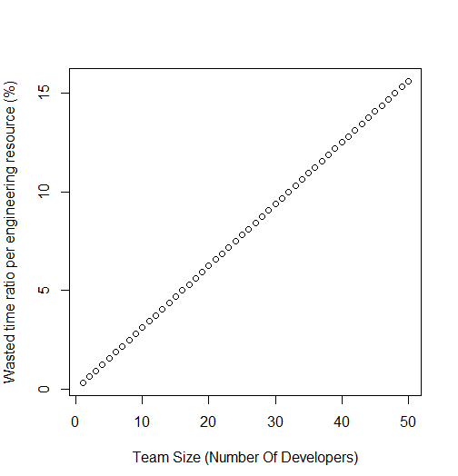
The following graph shows the expected waste time ratio for various team size. Interestingly, it’s linear relations.

Considering the benefit of CI, I would say less than 5% of blocking time is acceptable. According to the graph, therefore, it’s not something we should worry about until the team size becomes more than 16 developers.

I used the following R script for the calculation.

brokenPeriod  <- 0.5      # Build broken peirod = 30 min per week
devCount <- 1:50          # number of developers
downloadPerWeek <- 4 * 5  # Each developer refresh the source tree four times a day

wasteTimeF <- function(numOfDevs){
  blockedDownload <- 1:(numOfDevs * downloadPerWeek)
  totalDownload <- numOfDevs * downloadPerWeek
  p <- (brokenPeriod * numOfDevs) / 40
  
  sum(dbinom(blockedDownload, totalDownload, p) * (blockedDownload * brokenPeriod))
}

wasteRatioF <- function(numOfDevs){
  wasteTimeF(numOfDevs) / (numOfDevs * 40)
}

wasteRatio <- sapply(devCount, wasteRatioF) 
Posted in Algorithm, Statistics | Tagged , , , | Leave a comment

Windows thread pool keeps threads even after being closed

Windows Thread pool maintains threads so that it doesn’t have to create a new one when a work item is submitted. It may surprise you that it maintains threads even after you close the thread pool with CloseThreadpool() API function.

The following code demonstrates it. It starts 100 thread pool work items and monitors the number of threads in the process for the next 70 second. The thread pool object is closed immediately after posting the tasks.

LONG g_activeThreadCount = 0;

void CALLBACK WorkProc(PTP_CALLBACK_INSTANCE Instance, PVOID Context, PTP_WORK Work)
{
    InterlockedIncrement(&g_activeThreadCount);
    Sleep(5000);
    InterlockedDecrement(&g_activeThreadCount);
}

void PostThreadpoolWorks(int numberOfThreadpoolWorks)
{
    PTP_POOL pool = CreateThreadpool(NULL);
    if(!pool)
    {
        throw std::runtime_error("Fail to CreateThreadpool.");
    }

    PTP_WORK work = CreateThreadpoolWork(&WorkProc, NULL, NULL);
    if(!work)
    {
        CloseThreadpool(pool);
        throw std::runtime_error("Fail to CreateThreadpoolWork.");
    }

    for(int i = 0; i < numberOfThreadpoolWorks; i++)
    {
        SubmitThreadpoolWork(work);
    }

    CloseThreadpoolWork(work);
    CloseThreadpool(pool);
}

void Test1()
{
    // Post 100 thread pool work. The thread pool object is closed 
    // immediately.
    PostThreadpoolWorks(100);
    
    // keep monitoring the number of threads for 70 seconds.
    DWORD tick = GetTickCount();
    for(int i = 0; i < 100; i++)
    {
        cout << (GetTickCount() - tick) / 1000.0 << " " << GetNumOfThreads() << " " << g_activeThreadCount << endl;
        Sleep(1000);
    }
}

As each work item is finished in 5 seconds, the number of running threads (green) is 100 just for a few seconds. However, the number of threads in the process (red) is maintained for the next 68 seconds.

To confirm the observation, I started threads so that the number of running threads forms the triangle.

It indicates that the process maintains the maximum number of threads used within the last 65 to 70 seconds even though the thread pool object is closed.

Here is the program used in the experiment.

DWORD GetNumOfThreads()
{
    HANDLE hThreadSnap = INVALID_HANDLE_VALUE;
    THREADENTRY32 te32;

    hThreadSnap = CreateToolhelp32Snapshot(TH32CS_SNAPTHREAD, 0);
    if(hThreadSnap == INVALID_HANDLE_VALUE)
    {
        return (DWORD)-1;
    }

    te32.dwSize = sizeof(THREADENTRY32);
    
    if(!Thread32First(hThreadSnap, &te32))
    {
        CloseHandle(hThreadSnap);
        return (DWORD)-1;
    }
    
    DWORD count = 0;
    do
    {
        if( te32.th32OwnerProcessID == GetCurrentProcessId() )
        {
            count++;
        }
    } while( Thread32Next(hThreadSnap, &te32 ) );
    
    CloseHandle( hThreadSnap );
    return count;
}

LONG g_activeThreadCount = 0;

void CALLBACK WorkProc(PTP_CALLBACK_INSTANCE Instance, PVOID Context, PTP_WORK Work)
{
    InterlockedIncrement(&g_activeThreadCount);
    Sleep(5000);
    InterlockedDecrement(&g_activeThreadCount);
}

void PostThreadpoolWorks(int numberOfThreadpoolWorks)
{
    PTP_POOL pool = CreateThreadpool(NULL);
    if(!pool)
    {
        throw std::runtime_error("Fail to CreateThreadpool.");
    }

    PTP_WORK work = CreateThreadpoolWork(&WorkProc, NULL, NULL);
    if(!work)
    {
        CloseThreadpool(pool);
        throw std::runtime_error("Fail to CreateThreadpoolWork.");
    }

    for(int i = 0; i < numberOfThreadpoolWorks; i++)
    {
        SubmitThreadpoolWork(work);
    }

    CloseThreadpoolWork(work);
    CloseThreadpool(pool);
}

void Test1()
{
    // Post 100 thread pool work. The thread pool object is closed 
    // immediately.
    PostThreadpoolWorks(100);
    
    // keep monitoring the number of threads for 70 seconds.
    DWORD tick = GetTickCount();
    for(int i = 0; i < 100; i++)
    {
        cout << (GetTickCount() - tick) / 1000.0 << " " << GetNumOfThreads() << " " << g_activeThreadCount << endl;
        Sleep(1000);
    }
}

DWORD CALLBACK Test2Proc(LPVOID param)
{
    // Post some thread pool works for every 5 seconds.
    for(int i = 0; i < 10; i++)
    {
        PostThreadpoolWorks(i * 50);
        Sleep(5000);
    }
    for(int i = 10; i >= 0; i--)
    {
        PostThreadpoolWorks(i * 50);
        Sleep(5000);
    }
    return 0;
}

void Test2()
{
    // Start threads to post thread pool works.
    HANDLE hThread = ::CreateThread(NULL, 0, &Test2Proc, 0, 0, NULL);
 
    // keep monitoring the number of threads for 200 seconds.
    DWORD tick = GetTickCount();
    for(int i = 0; i < 200; i++)
    {
        cout << (GetTickCount() - tick) / 1000.0 << " " << GetNumOfThreads() << " " << g_activeThreadCount << endl;
        Sleep(1000);
    }

    CloseHandle(hThread);
}

int _tmain(int argc, _TCHAR* argv[])
{
    Test1();
    Test2();
	return 0;
}
Posted in Advanced Debugging, C++ | Tagged , | 1 Comment

std::unique_ptr for Windows handles

To close a Windows handle with std::unique_ptr, we need to define a type with operator() and specify it as the second template parameter.

struct Deleter
{
    // By defining the pointer type, we can delete a type other than T*.
    // In other words, we can declare unique_ptr<HANDLE, Deleter> instead of
    // unique_ptr<void, Deleter> which leaks the HANDLE abstraction.
    typedef HANDLE pointer;

    void operator()(HANDLE h)
    {
        if(h != INVALID_HANDLE_VALUE)
        {
            CloseHandle(h);
        }
    }
};

void OpenAndWriteFile()
{
    // Specify a deleter as a template argument.
    std::unique_ptr<HANDLE, Deleter> file(CreateFile(_T("test.txt"),
                                                     GENERIC_WRITE,
                                                     0,
                                                     NULL,
                                                     CREATE_ALWAYS,
                                                     FILE_ATTRIBUTE_NORMAL,
                                                     NULL));
    if(file.get() != INVALID_HANDLE_VALUE)
    {
        DWORD size;
        WriteFile(file.get(), "Hello World", 11, &size, NULL);
    }
}

This is different from std::shared_ptr where we can just specify the functor in a constructor parameter.

    std::shared_ptr<void> file(CreateFile(_T("test.txt"),
                                          GENERIC_WRITE,
                                          0,
                                          NULL,
                                          CREATE_ALWAYS,
                                          FILE_ATTRIBUTE_NORMAL,
                                          NULL),
                                CloseHandle);   // Specify deleter functor as a constructor parameter.

Although it’s extra work to define a new deleter type, std::unique_ptr has following advantage.

First, the smart pointer object doesn’t have to keep the deleter object, thus the size of the pointer becomes smaller. In fact, std::unique_ptr occupies the just same size as T*.

Second, Application can overwrite the pointer type. It means we can write:

std::unique_ptr<HANDLE, Deleter> foo(...);

instead of this HANDLE abstraction leakage version.

std::unique_ptr<void, Deleter> foo(...);
Posted in C++ | Tagged , | 4 Comments

HRD Emulator in HTML5

Just like MPEG-2 video uses VBV (Video Buffer Verifier), H.264 standard uses HRD (Hypothetical Reference Decoder) to define correctness of streams.

One of the verification provided by HRD is CPB buffer fullness. The idea is simple; feed H.264 stream to HRD and monitor the CPB fullness. Make sure the fullness never goes negative nor above the CPB buffer size. The importance of this buffer fullness requirement was explained here.

HRD defines the CPB fullness in somewhat counter intuitive way. To make it easy, I wrote an interactive HRD emulator in HTML5.

HRD Emulator (CBR)

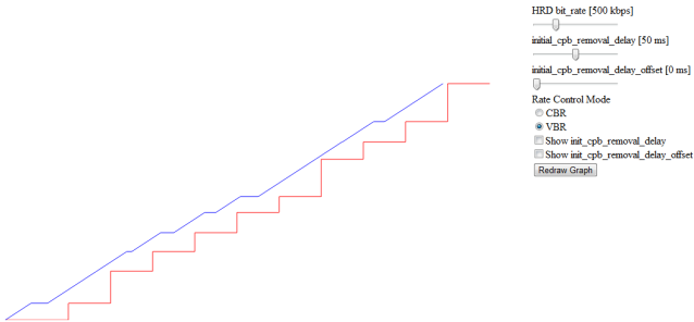
The blue line the number of bits entered to HRD over time. The input rate is constant in CBR mode, i.e. the blue line is straight. The red line is the number of bits removed (= Decoded) from CPB. Thus, the CPB fullness is the blue line minus the red line for a given time.

Let’s select the VBR in Rate Control Mode.

HRD Emulator (VBR)

HRD Emulator (VBR)

The blue line now has some periods where the input rate is zero. H.264 standard uses init_cpb_removal_delay to control the period; Bits for a picture N can enter HRD only after the picture decode time minus init_cpb_removal_delay.

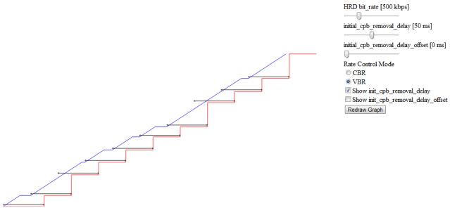
To see this rule more clearly, check “Show init_cpb_removal_delay” option. When the last bit of picture N – 1 arrives before the picture N decoding time minus init_cpb_removal_delay, the input rate goes down to zero.

HRD (VBR) with init_cpb_removal_delay

HRD (VBR) with init_cpb_removal_delay

The value of init_cpb_removal_delay also determines the initial decoding delay. It’s currently set to 50 ms. It means the first picture is decoded 50 ms after the first bit of the picture enters HRD.

The initial decoding delay determines the channel switching delay as discussed here. Can we reduce it to make channel switching faster?

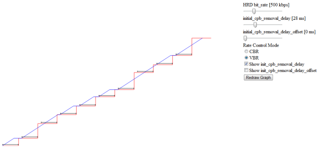
HRD underflow due to the short initial delay

Not really. As shown above, reducing the value of init_cpb_removal_delay resulted in the underflow error (the red line crosses the blue line).

H.264 standard has introduced another parameter to allow the reduction of initial decoding delay at the expense of increased average bit rate. Here we have init_cpb_removal_delay_offset parameter. It’s added to init_cpb_removal_delay for every picture except the first one.

HRD with non-zero init_cpb_removal_delay_offset

H.264 HRD provides these parameters to encoders so that they can choose optimal bit stream configuration for each target devices.

Here are HTML and Java Script of the HRD emulator above.

<html>
  <head>
    <title>HRD Emulator</title>
    <script src="./script.js" type="text/javascript"></script>
    
    <style type="text/css">
      #plot {
        float : left
      }
      #control-container {
        float : left
      }
      #widget {
        float : right;
        width : 10em
      }
      #heading {
        float : left
      }
    </style>    
  </head>
  <body onLoad="init()">
    <div id="plot">
      <canvas id="canvas" width="800" height="480"></canvas>
    </div>

    <div id="control-container">
      <div class="control">
        <div class="heading">HRD bit_rate [<span id="showBitRate"> </span> kbps]</div>
        <div class="widget">
          <input id="bitRate" onChange="update()" type="range" min="0" max="2000" value="500"/>
        </div>
      </div>
      <div class="control">
        <div class="heading">initial_cpb_removal_delay [<span id="showICRD"> </span> ms]</div>
        <div>
          <input id="initial_cpb_removal_delay" onChange="update()" type="range" min="0" max="100" value="50"/>
        </div>
      </div>
      <div class="control">
        <div class="heading">initial_cpb_removal_delay_offset [<span id="showICRDO"> </span> ms]</div>
        <div>
          <input id="initial_cpb_removal_delay_offset" onChange="update()" type="range" min="0" max="100" value="0"/>
        </div>
      </div>
      <div class="control">
        <div>Rate Control Mode</div>
        <div>
          <input type="radio" name="mode" value="cbr" onClick="setMode('cbr'); update()" checked="checked" />CBR
        </div>
        <div>
          <input type="radio" name="mode" value="vbr" onClick="setMode('vbr');  update()" />VBR
        </div>
      </div>
      <div class="control">
        <div>
          <input type="checkbox" id="isICRDVisible" onClick="update()"/>Show init_cpb_removal_delay
        </div>
      </div>
      <div class="control">
        <div>
          <input type="checkbox" id="isICRDOVisible" onClick="update()"/>Show init_cpb_removal_delay_offset
        </div>
      </div>
      <div class="control">
        <input id="reset" type="button" value="Redraw Graph" onClick="resetStream(); update();"/>
      </div>
    </div>
  </body>
</html>
// Save this as "script.js"
var canvas;
var picture = new Array();
var pictureDuration                  = 900900;
var initial_cpb_removal_delay        = 900900;
var initial_cpb_removal_delay_offset = 90090;
var cbr_flag = true;

function init()
{
    canvas = document.getElementById('canvas');
    resetStream();
    update();
}

function resetStream()
{
    var bit_rate = document.getElementById('bitRate').value * 1000;
    var averagePicSize = pictureDuration / 27000000 * bit_rate / 8;
    for(var i = 0; i < 10; i++){
        picture[i] = averagePicSize + (Math.random() - 0.5) * averagePicSize;
    }
}

function tickToX(tick)
{
    return tick / 900900 * 64;
}

function levelToY(level)
{
    return canvas.height - level / 50;
}

function drawDecodePictures(ctx)
{
    ctx.strokeStyle = 'rgba(255, 0, 0, 255)';

    ctx.beginPath();
    ctx.moveTo(0, levelToY(0));
    ctx.lineTo(tickToX(initial_cpb_removal_delay), levelToY(0));

    var prevX = tickToX(initial_cpb_removal_delay)
    var prevLevel = 0;
    for(var i = 0; i < 50; i++){
        var level = prevLevel + picture[i];
        var x1 = prevX;
        var x2 = prevX + tickToX(pictureDuration)
        var y  = levelToY(level);

        ctx.lineTo(x1, y);
        ctx.lineTo(x2, y);
        prevLevel = level;
        prevX     = x2
    }
    ctx.stroke();
}

function levelFromPeriod(period, bitRate)
{
    return period / 27000000.0 * bitRate / 8;
}

function drawInputData(ctx)
{
    var t_af          = new Array();
    var t_ai          = new Array();
    var t_ai_earliest = new Array();
    var t_rn          = new Array();

    var bit_rate = document.getElementById('bitRate').value * 1000;

    t_ai[0]   = 0;
    t_af[0]   = picture[0] * 8 * 27000000 / bit_rate;
    t_rn[0]   = initial_cpb_removal_delay;

    for(var n = 1; n < picture.length; n++)
    {
        t_rn[n] = t_rn[n - 1] + pictureDuration;
        if(cbr_flag == true)
        {
            t_ai[n] = t_af[n - 1];
        }
        else
        {
            t_ai_earliest = t_rn[n] - (initial_cpb_removal_delay + initial_cpb_removal_delay_offset);
            t_ai[n] = Math.max(t_af[n - 1], t_ai_earliest);
        }
        t_af[n] = t_ai[n] + picture[n] * 8 * 27000000 / bit_rate;
    }

    ctx.strokeStyle = 'rgba(0, 0, 255, 255)';
    ctx.beginPath();
    ctx.moveTo(tickToX(0), levelToY(0));

    var level = 0;
    for(var n = 0; n < picture.length; n++)
    {
        ctx.lineTo(tickToX(t_ai[n]), levelToY(level));
        level += picture[n];
        ctx.lineTo(tickToX(t_af[n]), levelToY(level));
    }
    ctx.stroke();

    level = 0;
    for(var n = 0; n < picture.length; n++)
    {
        var isICRDVisible = document.getElementById("isICRDVisible").checked;
        if(isICRDVisible){
            // draw initial_cpb_removal_delay period
            var icrd_x1 = tickToX(t_rn[n] - initial_cpb_removal_delay)
            var icrd_x2 = tickToX(t_rn[n])
            var icrd_y  = levelToY(level) - 4

            ctx.strokeStyle = 'rgba(0, 0, 0, 255)';
            ctx.beginPath();
            ctx.moveTo(icrd_x1, icrd_y);
            ctx.lineTo(icrd_x2, icrd_y);
            ctx.stroke();

            ctx.beginPath();
            ctx.moveTo(icrd_x1 + 2, icrd_y - 2);
            ctx.lineTo(icrd_x1, icrd_y);
            ctx.lineTo(icrd_x1 + 2, icrd_y + 2);
            ctx.stroke();

            ctx.beginPath();
            ctx.moveTo(icrd_x2 - 2, icrd_y - 2);
            ctx.lineTo(icrd_x2, icrd_y);
            ctx.lineTo(icrd_x2 - 2, icrd_y + 2);
            ctx.stroke();
        }

        var isICRDOVisible = document.getElementById("isICRDOVisible").checked;
        if(isICRDOVisible){
            // draw initial_cpb_removal_delay period
            var icrdo_x1 = tickToX(t_rn[n] - initial_cpb_removal_delay - initial_cpb_removal_delay_offset)
            var icrdo_x2 = icrd_x1
            var icrdo_y  = levelToY(level) - 4

            ctx.strokeStyle = 'rgba(0, 0, 0, 255)';
            ctx.beginPath();
            ctx.moveTo(icrdo_x1, icrdo_y);
            ctx.lineTo(icrdo_x2, icrdo_y);
            ctx.stroke();

            ctx.beginPath();
            ctx.moveTo(icrdo_x1 + 2, icrdo_y - 2);
            ctx.lineTo(icrdo_x1, icrdo_y);
            ctx.lineTo(icrdo_x1 + 2, icrdo_y + 2);
            ctx.stroke();

            ctx.beginPath();
            ctx.moveTo(icrdo_x2 - 2, icrdo_y - 2);
            ctx.lineTo(icrdo_x2, icrdo_y);
            ctx.lineTo(icrdo_x2 - 2, icrdo_y + 2);
            ctx.stroke();
        }
        level += picture[n];
    }
}

function setMode(mode)
{
  cbr_flag = mode == "cbr";
}

function updateUI(uiName, valueName)
{
    document.getElementById(uiName).innerHTML = document.getElementById(valueName).value
}

function update()
{
    var ctx    = canvas.getContext('2d');
    ctx.fillStyle = 'rgba(255, 255, 255, 255)';
    ctx.fillRect(0, 0, canvas.width, canvas.height);

    updateUI("showBitRate", "bitRate");
    updateUI("showICRD", "initial_cpb_removal_delay");
    updateUI("showICRDO", "initial_cpb_removal_delay_offset");

    initial_cpb_removal_delay = document.getElementById('initial_cpb_removal_delay').value * 27000;
    initial_cpb_removal_delay_offset = document.getElementById('initial_cpb_removal_delay_offset').value * 27000;

    drawDecodePictures(ctx);
    drawInputData(ctx);
};
Posted in Video | Tagged , , , , | 1 Comment